5 Uncertainty and data quality information
5.1 Overview
This section is a summary of section “Data uncertainty” in the ATBD. The basic principle of the uncertainty and data quality information in the PGN data products is this:
Those error sources, which we can quantitatively propagate through the retrieval algorithm, are included in the output uncertainty of the L2 data (Section 5.2).
Those error sources, which we know exist, but we cannot quantify, are either included in the DQF of the L2 data (Section 5.4), or not included at all (Section 5.5).
Hence to distinguish between “good” and “bad” data, both the uncertainty output and the DQF should be used. As already mentioned in Chapter 2, only the L2 data in observation mode have a complete set of uncertainties as described in Section 5.2. Those measured in observation mode Profile have a more limited uncertainty information.
5.2 Uncertainty types
Three types of uncertainties are distinguished, which differ from each other by the correlation length in time:
Independent uncertainty : the correlation length in time is zero. An example is the photon noise propagated into the TotCol measured at a certain moment, which is totally uncorrelated to the propagated photon noise for measurements taken at any other time.
Common uncertainty : the correlation length in time is infinite. An example is an error in the assumed slant column in the reference spectrum. This error affects all retrieved columns using the same reference spectrum in the same way, hence the error at a certain measurement is fully correlated to the error for measurements taken at any other time.
Structured uncertainty : the correlation length in time is larger than zero, but not infinite. An example is a difference between the effective temperature of a trace gas used in the spectral fitting (assuming that the temperature is NOT fitted itself) and the true effective temperature of this gas in the atmosphere. This introduces an error in the retrieved column, which is highly correlated to measurements taken around the same time, but in general not correlated to measurements taken at times farther away. E.g. if an effective ozone temperature of 225 K is used in the spectral fitting, but the true effective ozone temperature is 228 K at 10:00 in the morning of 27 October, this causes approximately a -1% error in the retrieved ozone slant column. The next measurement on this day at 10:02 will still suffer nearly exactly the same error, since the true temperature has hardly changed in the 2 minutes. However a few days later, on 3 November, the true temperature has in general changed and might be 225 K, which means the error due a mismatch of the effective temperature is then 0 and not correlated to the error from 27 October at 10:00.
For the total uncertainty U of a single data point, we simply combine U\(_\text{I}\), U\(_\text{C}\) and U\(_\text{S}\) as shown in Equation 5.1:
\[\text{U} = \sqrt{\text{U}_\text{I}^2 + \text{U}_\text{C}^2 + \text{U}_\text{S}^2} \tag{5.1}\]
When the data are averaged, e.g. by building the mean TotCol over a certain time interval, the combined uncertainty associated with the mean is a combination of the individual U\(_\text{I}\)(i), U\(_\text{C}\)(i) and U\(_\text{S}\)(i). i=1 to n is the index for a single data point out of the n data points averaged. Here we look at the two “extreme” cases.
In the first situation the structured errors are fully correlated along the dimension. In this “short” case the total uncertainty of the mean value, called U(n,short), is given by:
\[\text{U(n,short)} = \frac{1}{\text{n}} \cdot \sqrt{ \sum_{i=1}^{\text{n}} \left[ \text{U}_\text{I}\left(\text{i}\right)^2 \right] + \left[ \sum_{i=1}^{\text{n}} \text{U}_\text{C}\left(\text{i}\right) \right]^2 + \left[ \sum_{i=1}^{\text{n}} \text{U}_\text{S}\left(\text{i}\right) \right]^2 } \tag{5.2}\]
Hence the independent uncertainty of the mean is “reduced” compared to the individual values, but the common and structured uncertainties are not. An example for this would be the mean TotCol over a rather short time period, e.g. 10 min, in which we assume the data with respect to mismatch of the true and assumed effective trace gas temperature to be fully correlated.
The other extreme case assumes the structured uncertainties to be uncorrelated along the dimension. In this “long” case the total uncertainty U(n,long), is given by:
\[\text{U(n,long)} = \frac{1}{\text{n}} \cdot \sqrt{ \sum_{i=1}^{\text{n}} \left[ \text{U}_\text{I}\left(\text{i}\right)^2 \right] + \left[ \sum_{i=1}^{\text{n}} \text{U}_\text{C}\left(\text{i}\right) \right]^2 + \sum_{i=1}^{\text{n}} \left[ \text{U}_\text{S}\left(\text{i}\right)^2 \right]} \tag{5.3}\]
Here the structured uncertainty “behaves” like the independent uncertainty. An example for this would be the mean TotCol over a long time period, e.g. one year, when we assume that the temperature used in the spectral fitting is from a climatology that represents very well the average true effective temperature over this year. Then we could say that the temperature errors are a mixture of over- and underestimations and can therefore be approximated as uncorrelated overall.
5.3 Total uncertainty for operational direct sun products
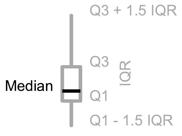
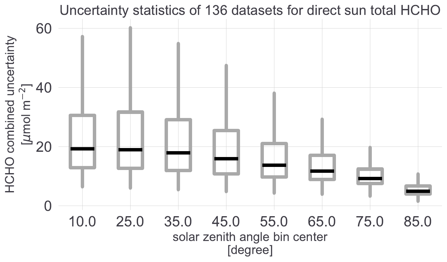
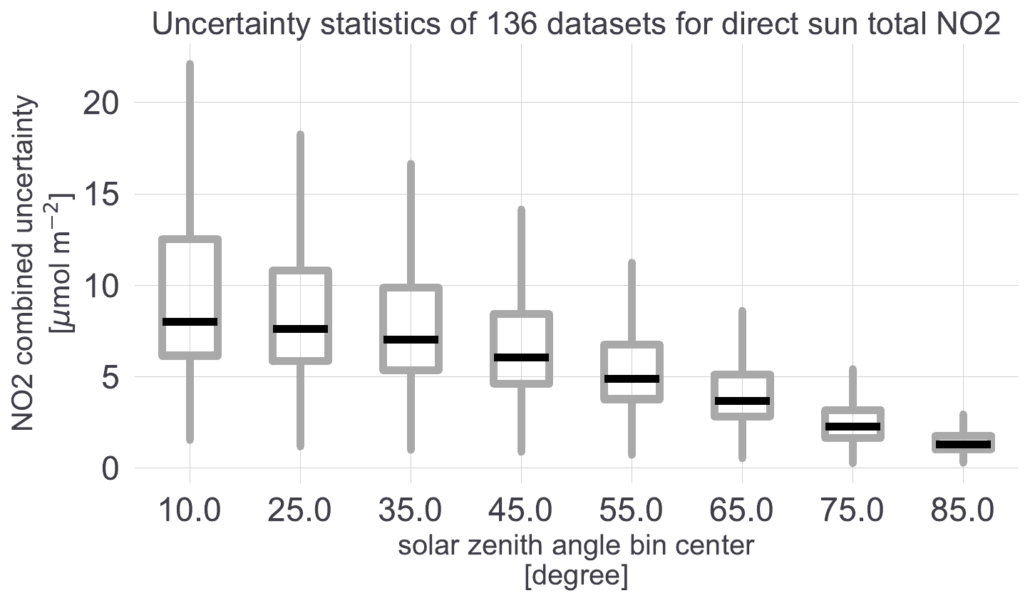
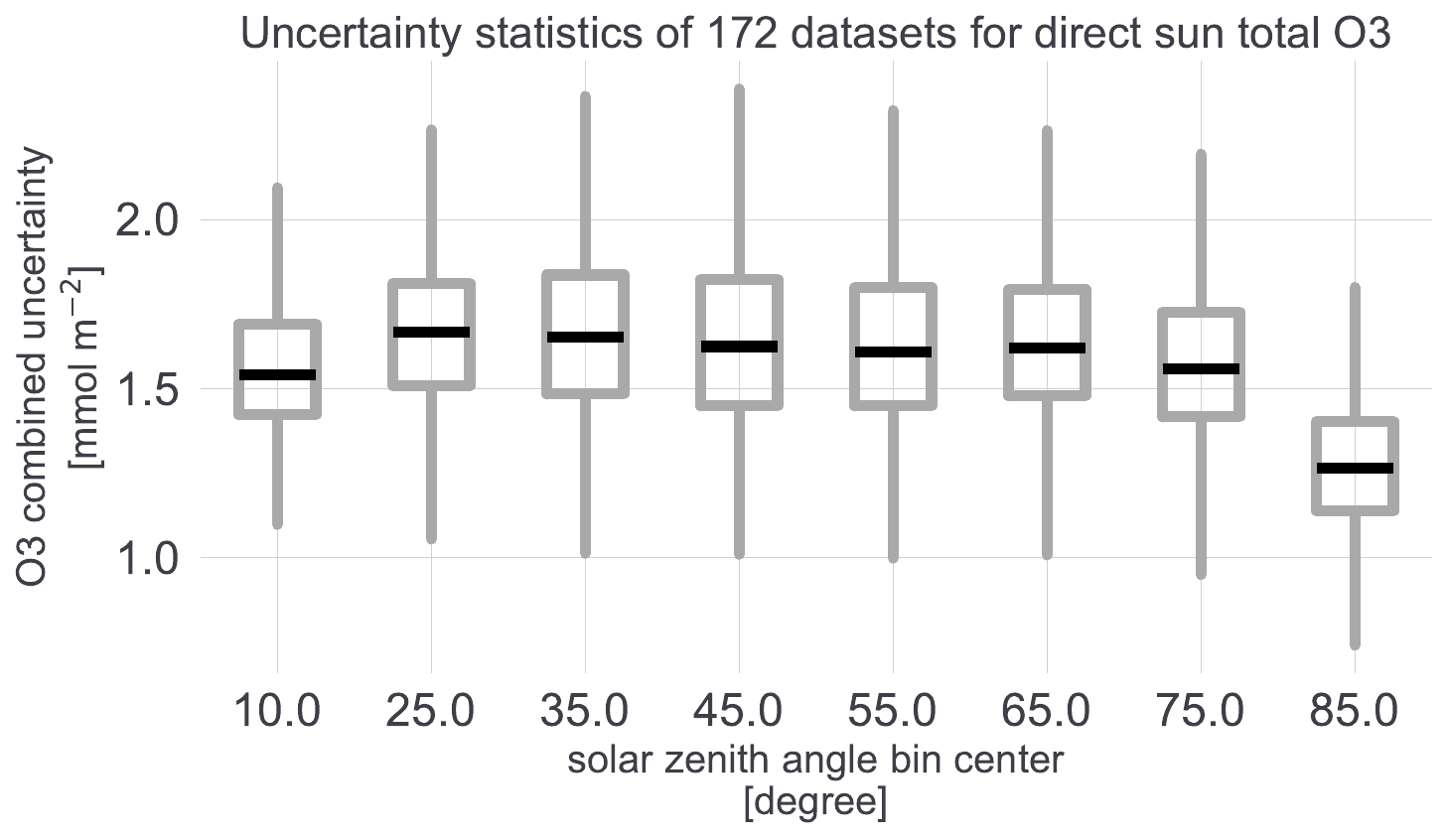
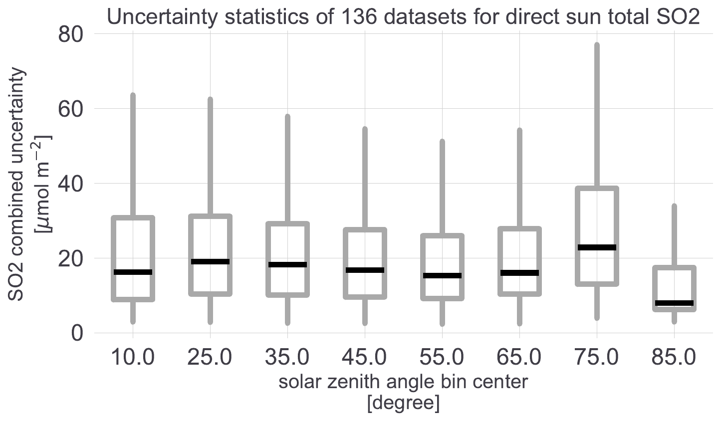
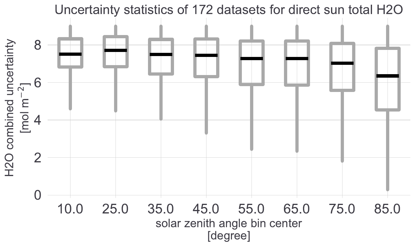
Based on the available PGN data from January 16 2025, we have calculated the total uncertainty (Equation 5.1) for all operational products at that time. As the SZA has a strong influence on the total uncertainty, we have binned the data accordingly, considering only high quality data. Each SZA bin is summarized as a box-plot with the box and whiskers as defined in the legend on the right (Q1=1 quartile (25%), IQR=inter-quantile-range). Table 5.1 provides a guide to the individual plots.
| Product | Version | Figure | Data unit | Datasets |
|---|---|---|---|---|
| HCHO TotCol | rfus5p1-8 | Figure 5.1 | \(\mu\)mol m\(^{-2}\) | 136 |
| NO2 TotCol | rnvs4p1-8 | Figure 5.2 | \(\mu\)mol m\(^{-2}\) | 136 |
| O3 TotCol | rout2p1-8 | Figure 5.3 | mmol m\(^{-2}\) | 172 |
| SO2 TotCol | rsus1p1-8 | Figure 5.4 | \(\mu\)mol m\(^{-2}\) | 136 |
| H2O TotCol | rwvt1p1-8 | Figure 5.5 | mol m\(^{-2}\) | 172 |
5.4 Data Quality Flags
Currently there are 9 possible DQFs: DQ0, DQ1, DQ2, DQ10, DQ11, DQ12, DQ20, DQ21 and DQ22. The unit position 0, 1 or 2 has the following meaning:
Unit position 0, “High quality”: no data quality indicator exceeds the data quality 1 (DQ1) limit and therefore there are no indications that the data might not be of the highest possible quality. Once quality assured, those data can be used with high confidence and the uncertainty associated with these additional effects is negligible, i.e. the provided uncertainty can be assumed to represent the true uncertainty.
Unit position 1, “Medium quality”: at least one data quality indicator exceeds the DQ1 limit and therefore the quality of the data might be reduced. Depending on the application, the user should decide whether to use these data. Note that the reduced quality can originate from instrumental sources (e.g. too large wavelength shift) or atmospheric sources (e.g. clouds in direct sun measurements). This also means that the reported data underestimates the true uncertainty by a small amount.
Unit position 2, “Low quality”: at least one data quality indicator exceeds the data quality 2 (DQ2) limit and therefore the quality of the data is strongly reduced. For most purposes, the user should not use these data. As for unit position 1, the low quality can originate from instrumental or atmospheric sources. In this case it is nearly certain that reported data uncertainty underestimates the true uncertainty.
The decade of the DQF can be 0, 1 or 2 and has the following meaning:
Decade 0, “Quality assured”: this means that quality control (QC) has already been applied to the data. QC consists of a semi-automatic inspection of the obtained L2 data to determine, whether the instrument was monitoring correctly over a certain measurement period. With this procedure one can possibly detect factors influencing the data quality, which are not reflected in the uncertainty and not captured by the DQF. An example would be a dirty entrance window. This reduces the overall throughput of the system and is interpreted by the algorithm as an increased aerosol load in the atmosphere. Since this effect causes usually a non-physical dependence of the AOD on the solar ZA, it can often be detected in the QA process. After the QC has been performed, the unit position will not change anymore.
Decade 1, “Not quality assured”: the quality flag in the unit position is based on an initial estimate and formal QC has not been carried out. It is possible that the unit position changes after that happens.
Decade 2, “Unusable data”: this means the data are not usable, which can have the following reasons: The QC has revealed that there were data quality issues during that time. r-code entry “Product status” says “unusable” for the respective output gas. This is typically the case for a trace gas that is not the “primary” gas to be fitted, for which the fitting setup, especially the wavelength range, is not optimized. These data will not undergo QC.
The synthetic reference spectrum is used, but no calibration was applied to it. These data will not undergo QC.
It is also important to note, that the unit position of the DQF can only stay the same or increase through the different processing levels, but never go down.
5.5 Not covered by uncertainty or DQF
The following list describes effects, which are not included in the uncertainty output or the DQF, but we know that they can contribute to the data uncertainty. It is planned that these effects are included in the future. Obviously it is also possible that other effects, which are unknown to us and therefore not listed here, may contribute to the uncertainty.
Cross sections: Neither the choice of the cross sections nor their uncertainty is currently taken into account.
Algorithm: The spectral fitting algorithm is an approximation and “suffers” from intrinsic deficiencies. Those are mostly caused by the use of pre-convoluted parameters, e.g. the cross sections, and cross-correlation among the fitted parameters. These effects are not considered in the current software version.
Spectral fitting quality: Although the spectral fitting residual RMS is used as a threshold in the DQF, its impact on the uncertainty is not considered.
Theoretical reference spectrum: Any systematic issues arising from using this reference not measured by the instrument itself are neglected.